Markov Chains
The Math behind the various transitions of Markov Chains


Markov Chains
- Markov chains are the combination of probabilities and matrix operations
- They model a process hat proceeds in steps (time, sequence, trails, etc.); like serires of porbability trees
- The model can be in opne "state" at each step
- When the next setp occurs, the porcess can be in the same state or move to another state.
- Movements between states are defined by porbabilites
- All probabilites exiting a state must add up ot 1
- We can then find the probabilites of being in any given state many steps into the process
- ref: https://www.youtube.com/channel/UCFrjdcImgcQVyFbK04MBEhA
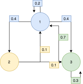
The Tranistion Matrix for the above State Transition Diagram:
\begin{equation*} To \\ From \begin{bmatrix} 1 \rightarrow 1 & 1 \rightarrow 2 & 1 \rightarrow 3 \\ 2 \rightarrow 1 & 2 \rightarrow 2 & 2 \rightarrow 3 \\ 3 \rightarrow 1 & 3 \rightarrow 2 & 3 \rightarrow 3 \end{bmatrix} \end{equation*}\begin{equation*} To \\ From \begin{bmatrix} .2 & .4 & .4 \\ .1 & 0 & .9 \\ .7 & 0 & .3 \end{bmatrix} \end{equation*}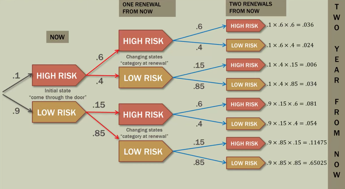
# one step conditional transition matrix
# [[High to High; High to Low],
# [Low to High; Low to Low]]
tm = np.array([
    [.6, .4],
    [.15, .85]
])
# Initial State Vector which says picking at random,
# 10% areunder 'High Risk' and 90% are under 'Low Risk'
# [[High; Low]]
isv = np.array([
    [.1, .9]
])
# Now we want to find th porbabilites of
# high and low one year from now we multiply those together.
# Initial State Vector * Transition Matrix
one_year_pHL = np.dot(isv, tm)
print(one_year_pHL)
Now we have the Probabilities of High risk and Low risk one year from now. So, If a new customer renews after one year, the porbability he/she is High Risk or Low Risk is .195 and .085 respectively
# One_step_Transition_vector * Transition_matrx
np.dot(one_year_pHL, tm)
We can see here, our high-risk group has a probability of 0.2377 and our low risk probability is 0.7622 which add up to one.
Now, in a practical sense we can really see here just much higer risk our drivers are than the general population, so a new dirver comes into our office to signup and after two years we can see the probability of being high-risk is 0.2377.
If a new customer renews after two years, the probability he/she is High Risk or Low risk is 0.2377 and 0.7622 respectively
# initial_state_vector * transition_matrix^2
np.dot(isv, np.dot(tm,tm))
We can use the initial State vector constant and perfome square for the transition matrix for two step transition to perform three step transition we can perfome cube of the transition matrix. ransition probability values of Hight Risk and Low risk
Here for getting two step transition probability values of Hight Risk and Low risk inital_state_vecot transition_matirx2 == one_step_transition_prob_values * transitio_matrix
np.dot([[1, 0]], np.dot(tm, tm))
# considering only for High Risk:
h_hl_hl_sum = .036+.024+.006+.034
h_hl_h_sum = .036+.006
h_hl_l_sum = .024+.034
print("Customer's High Risk",h_hl_h_sum/h_hl_hl_sum)
print("Customer's Low Risk", h_hl_l_sum/h_hl_hl_sum)
If a customer is placed in the Low Risk category when they sign up, what is the probability that customer will be High Risk or Low Risk two years from now?
np.dot([[0, 1]], np.dot(tm, tm))
l_hl_hl_sum = .081+.054+.11475+.65025
l_hl_h_sum = .081+.11475
l_hl_l_sum = .054+.65025
print(l_hl_h_sum/l_hl_hl_sum)
print(l_hl_l_sum/l_hl_hl_sum)
$$[Initial State Vector][Transition Matrix]^m = [m - State Probabilities]$$
State probabilites m years from now
from numpy import linalg
powers = [2, 3, 5, 10, 20, 25, 30, 40]
for po in powers:
    print("isv * transition_matrix^{}".format(po),np.dot(isv, linalg.matrix_power(tm, po)))
Here we are changing the number of years in to the future we are intrested in, when we got down to 20 years into the future and then we did for 25, 30... Notice the porbabilites seemed to have stablilized they steadied out, NO matter how many more years and of the future we went they didn't change they stoped changing.
This is called Steady-State Vectors
Eventually, continuing to multiply our answer by the transition matrix again has no effect on the outcome. Twenty-five years in the future is the same as 50 years into the future, etc., $$v_{\infty}P = v_{\infty}$$
General Steady State Vectors: $$vP = v$$
- $v$ Initial State Matrix
- $P$ Transition Matrix
print(np.dot([[0.2727, 0.7273]], tm))
$$[.6x+.15y \ \ .4x+.85y] = [x \ y]$$ $$.6x+.15y = x \\ .4x+.85y = y$$ $$-.4x+.15y=0 \\ .4x-.85y = 0 $$ If we mulitply one of the equaitons by $-$ both the equations are same .Since the equaitons are identical, we can make them into one. $$.4x-.15y = 0 \ \ \ -eq(1)$$ Now, we know that the initial state vector has to equal to 1 so, what ever $x$ is and what ever $y$ is they have to add up to 1 $$x+y = 1 \ \ \ -eq(2)$$ By solving eq(1) and eq(2), $$x = \frac{.15}{.55} = 0.2727 \\ y = \frac{3}{11} = .7273$$
\begin{gather} \begin{bmatrix} \frac{3}{11} & \frac{8}{11} \end{bmatrix} \dot{} \begin{bmatrix} .6 & .4 \\ .15 & .85 \end{bmatrix}= \begin{bmatrix} \frac{3}{11} & \frac{8}{11} \end{bmatrix} \end{gather}Method 2: $$vP = v \\ vP-v = 0 \\ v(P-1)=0$$ In matrix mulitplication an identity matrix $I$ is the equvilent of $1$; $v.I=v$ $$v(P-I) = 0$$ By using Gaussian method of solving equations, we can obatin x and y values which which in return are same as above
A reluctant gambler is dragged ot the riverboat casino by his more free-wheeling friends. He takes only \$50\ ot gamble with.
Since he doesnot know much about gamling, he decides to play roulette. At each spin, he places \$25 on red. If red occurs, he wins \$25. If black comes up, he loses his \$25. Therefore the odds of winning are 50% (it's lower in the actual game.)
He will quit playing when he either has zero money left, or is up \$25(\$75 total).
Let's model this process as a Markov Chain and examine its long-run behavior.
\begin{equation*} \$0\ \$25 \ \$50 \ \$75 \\ \$0\ \$25 \ \$50 \ \$75 \begin{bmatrix} 1 & 0 & 0 & 0 \\ .5 & 0 & .5 & 0\\ 0 & .5 & 0 & .5 \\ 0 & 0 & 0 & 1 \end{bmatrix} \end{equation*}Let's consider $P$ as the above state transition matrix. When we run this process many steps in the future.
import numpy as np
p = np.array(
    [[1, 0, 0, 0],
    [0.5, 0, 0.5, 0],
    [0, 0.5, 0, 0.5],
    [0, 0, 0, 1]])
linalg.matrix_power(p,2)
linalg.matrix_power(p,10)
linalg.matrix_power(p,25)
$$P^{\infty} = [x \ \ 0 \ \ 0 \ \ (1-x)]$$
The Gambler started with \$ 50$; which is state 3. Therefore we can set up an inital state vector that look like this: $$v = \begin{bmatrix} 0 & 0 & 1 & 0 \end{bmatrix}$$
v50 = np.array([[0, 0, 1, 0]])
v50.shape
np.dot(v50, linalg.matrix_power(p, 50))
If the Gambler started with \$25$ he would begin in state 2. Therefore we can set up aninitial vector that looks like this $$v = \begin{bmatrix} 0 & 1 & 0 & 0 \end{bmatrix}$$
v25 = np.array([[0, 1, 0, 0]])
v50.shape
np.dot(v25, linalg.matrix_power(p, 50))